How To Calculate Running Average In Excel

So, there I was, staring at a spreadsheet that looked like it had been through a paper shredder and then glued back together by a mischievous toddler. Numbers were everywhere, each one screaming "I'm important!" but I had no idea how to make sense of them. That's when I remembered the magical world of running averages. You know, those sneaky little numbers that follow you around like a faithful hound, always ready to give you the most up-to-date info.

Now, I'm not a math whiz by any stretch. I mean, I can count my change at the grocery store, but that's about as far as my numerical prowess goes. But I've learned a thing or two about Excel over the years, and I'm here to tell you that calculating a running average is easier than you think. So, grab your coffee (or tea, I don't discriminate), and let's dive in.

What's a Running Average, Anyway?

Alright, let's start with the basics. A running average is like a moving average, but instead of looking at a fixed number of periods, it keeps track of the average as new data comes in. In other words, it's always looking forward, ready to adapt to new information. Think of it like a weather forecast that updates every hour - it's not just giving you the average temperature for the day, it's telling you what's happening right now.

In the context of our spreadsheet, let's say we're looking at daily sales figures. A running average would give us the average sales for the current day, plus all the days before it. So, if we're on day 5, our running average would be the average of days 1 through 5.

Let's Get Our Hands Dirty

Alright, enough talking. Let's get into the nitty-gritty. I'm going to assume you've got your data laid out in a simple column. Let's call this column "Sales" and it's in column B, starting from row 2 (because row 1 is usually where our headers are).

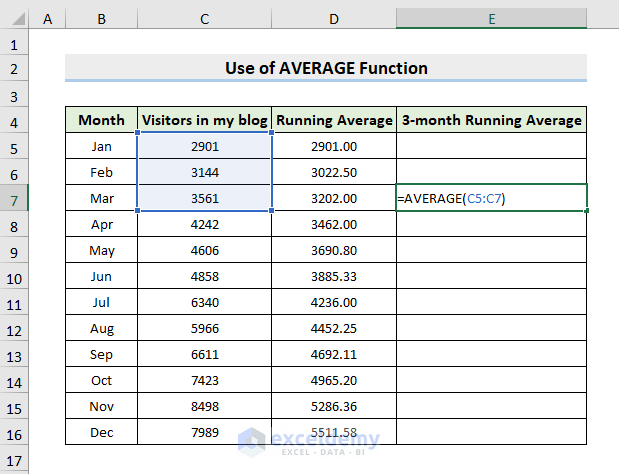
Now, here's where the magic happens. In cell C2, we're going to type in the following formula:

How to Calculate Running Average in Excel (6 Suitable Ways) - Excel Insider

=AVERAGE(B$2:B2)

Let me break that down for you. =AVERAGE is the function we're using to calculate the average. B$2:B2 is the range of cells we're averaging. The dollar sign ($) before the 2 in B$2 is important - it makes that cell a absolute reference, so it won't change as we drag the formula down.

Now, drag that formula down as far as you need to go. Each cell will now show the running average up to that point. Easy peasy, right?

But Wait, There's More!

What if you want to see the running average for every 7 days, not every day? No problem! Just change the range in our formula to =AVERAGE(B$2:B2-B$2+7). This will give us the average for the current day and the 6 days before it.

How to Calculate Running Average in Excel (6 Suitable Ways) | Excel Insider

And if you want to see the running average for every 30 days, just change the number to 30. See how flexible this is?

Final Thoughts

And there you have it! Calculating a running average in Excel is like learning to ride a bike. Once you get the hang of it, you'll be zooming around like a pro. Just remember, the key is to use absolute references so your range stays put.

So, the next time you're staring at a spreadsheet, wondering how to make sense of all those numbers, give running averages a try. You might just find that they're the key to unlocking the insights you've been looking for.

Now, go forth and average! And remember, if you get stuck, there's no shame in asking for help. We've all been there, staring at a spreadsheet, wondering what on earth those numbers are trying to tell us.