How To Reverse Order Of Columns In Excel

Hey there, spreadsheet whiz! Ever found yourself staring at an Excel sheet, wishing you could flip those columns like you're flipping through a magazine? I feel ya. Today, we'...
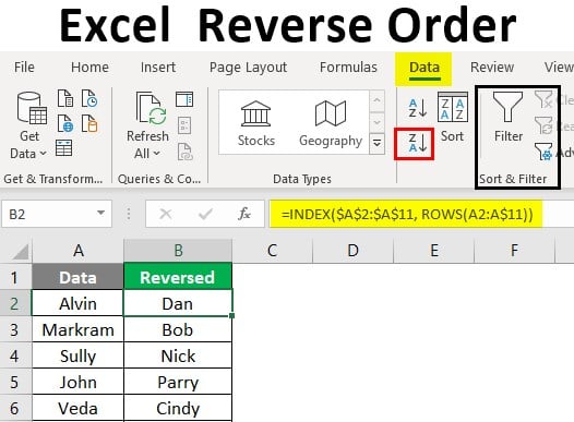
Hey there, spreadsheet whiz! Ever found yourself staring at an Excel sheet, wishing you could flip those columns like you're flipping through a magazine? I feel ya. Today, we're gonna chat about how to reverse the order of columns in Excel. Grab your coffee, let's dive in!
Why Reverse Columns?
Now, you might be thinking, "Why on earth would I want to do that?" Well, my friend, there are times when you need to see your data from a different angle. Maybe you've got a long list of sales figures, and you want to compare January's performance with December's. Reversing columns can make that a breeze!
Or maybe you're just one of those people who likes to shake things up a bit. I mean, who said columns have to be in order, right? Let's mix things up!
Must Read
Method 1: The Simple Sort
Alright, let's start with the easiest method. This one's so simple, even your grandma could do it. (No offense, Grandma.)
- Select the columns you want to reverse. Don't forget to hold down Ctrl (or Cmd on Mac) to select multiple columns.
- Right-click on any of the selected columns and choose Sort – or just press Alt + A + S.
- In the Sort dialog box, under Column, choose the column you want to sort by. Then, under Sort On, choose Cell Color. Click OK.
Voila! Your columns should now be reversed. The catch? This method only works if your columns have different background colors. If they're all the same, you'll need to change them first. But hey, that's a fun excuse to add some color to your spreadsheets!
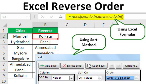 Excel Tutorial: How To Reverse The Order In Excel – QWFNTW
Method 2: The Insert Rows Trick
Now, let's try something a bit more sneaky. This method involves inserting rows and then deleting them in a specific order. It's like a magic trick for your data!
- Select the columns you want to reverse.
- Right-click and choose Insert – or just press Ctrl + +.
- Delete the new row you just inserted. But here's the trick: instead of just clicking the row number, click the little square at the top left of the row. This will delete the entire row, along with its contents.
- Repeat steps 2 and 3 until all your columns are reversed. It's like a little dance, isn't it?
And there you have it! Your columns should now be reversed, and you've learned a new trick to impress your coworkers. (Or scare them. I won't judge.)
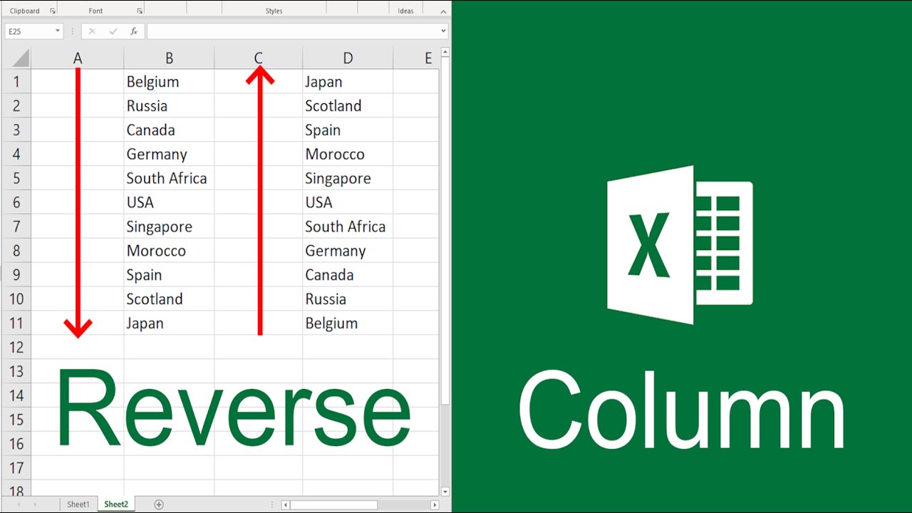 Flip Chart Upside Down Excel at Antoinette Roy blog
Bonus Tip: Freeze Those Rows!
Alright, one more thing before we wrap up. When you're reversing columns, it's easy to lose track of your headers. To keep them in place, you can freeze the top row. Here's how:
- Click on the row below your headers.
- Go to the View tab, then click on Freeze Panes – or just press Alt + F.
- Choose Freeze Top Row. Now your headers will stay put, no matter how many times you reverse those columns!
And that's a wrap, folks! I hope you've enjoyed our little chat about reversing columns in Excel. Remember, spreadsheets don't have to be boring. Mix things up, have some fun, and who knows? You might just find a new way to make your data dance!
Until next time, happy reversing!
